Answer the question
In order to leave comments, you need to log in
How to write a formula in excel that will highlight cells if the price in them is less than in the first column?
That is, it is necessary for excel to compare the numbers from the first column with others, and if they are lower than in the first column, highlight these cells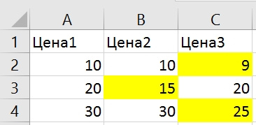
Answer the question
In order to leave comments, you need to log in
Conditional Formatting > Highlight Rule > Less Than You
specify which column is less than. In your case, A2
And so for B2 and C2
Then stupidly select B2 + C2 and drag the cross down;)
Let's say you need to select cells in the range B1:I25, comparing them with the prices in column A (see screenshot)
1. select the range B1:I25
2. Tab Home -> Conditional formatting -> Less than
3. In the "Format cells that are less than" field: " put the cursor and click on cell A1 - the entry = $ A $ 1 will appear
4. Change it to = $ A1 either manually or by pressing the F4 key.
5. Click OK
6. PROFIT!!!
Let me explain the principle of operation: Initially, conditional formatting is applied to the first cell in the selected range (in our case, B10) and then the rule is transferred to the entire selected range, taking into account the absolute / relativity of the reference to the cell specified in the rule (cell A1). Because when shifting along a column, we need to compare everything with the same column A, we fix it with the $ symbol, but since when shifting one line down, we need to compare not with A1 but with A2, then the $ sign must be removed before 2.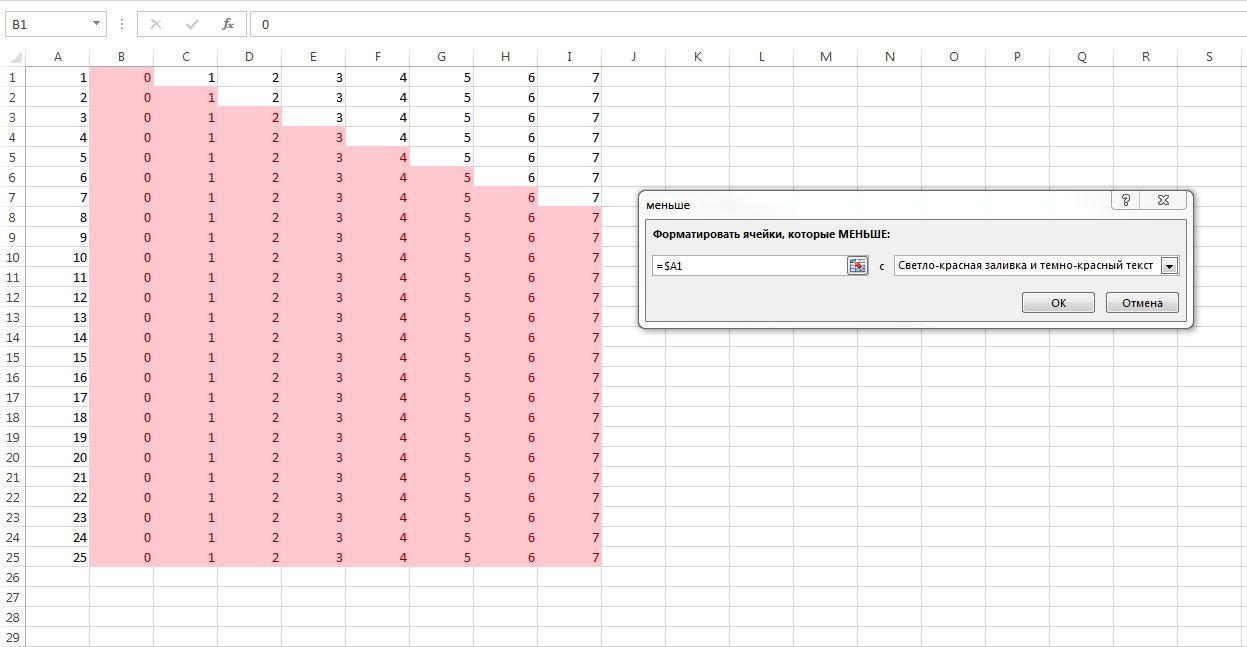
Didn't find what you were looking for?
Ask your questionAsk a Question
731 491 924 answers to any question