How to use "cell value=sheet title" formula in VLOOKUP range?

Question

Google Sheets

In cell B1, the text is in the form of a date range.
B1="18.01-25.01"
There are also sheets named after these intervals.
Sheet1 = 18.01
Sheet2 = 25.01
I wanted to take data from these sheets through VLOOKUP and display the difference between the values ​​of Sheet2 and Sheet1, but since cell B1 is dynamic, I inserted a formula (LEFT and RIGHT) into the range, but it does not work ...
Example below:
=VLOOKUP(A3;"'"RIGHT(B1;5)"'!A:C";2;FALSE)-VLOOKUP(A3;"'"LEFT(B1;5)"'!A:C";2; FALSE)
"'"RIGHT(B1;5)"'!A:C" - range A:C in sheet 25.01 and in the formula it should be displayed as '25.01'!A:C
How to implement this?

Answer 1

Without an example, it's hard to say what you actually need, but for me

=VLOOKUP(A3;INDIRECT(INDEX(SPLIT(B1;"-");1;1) &"!A:C");2;FALSE)
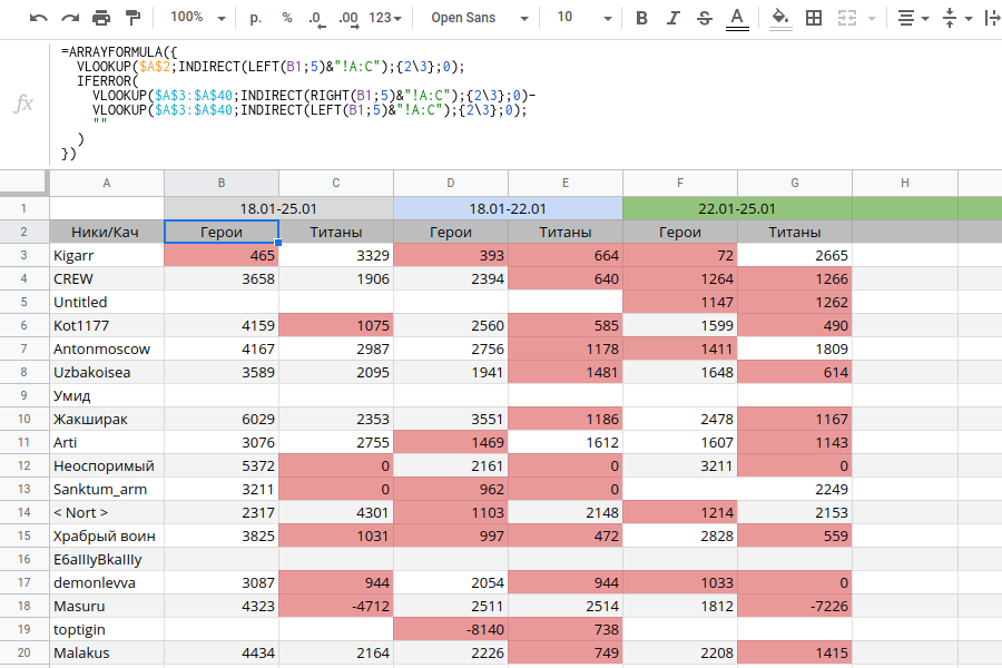
-VLOOKUP(A3;INDIRECT(INDEX(SPLIT(B1;"-");1;2) &"!A:C");2;FALSE)

works well. INDEX can be replaced with your LEFT/RIGHT expressions.
UPDATED
Thanks for the example. He helped a lot. I would choose the following way: add a formula for the entire date range at once. For example,

=ARRAYFORMULA({
  VLOOKUP($A$2;INDIRECT(LEFT(B1;5)&"!A:C");{2\3};0);
  IFERROR(
    VLOOKUP($A$3:$A$40;INDIRECT(RIGHT(B1;5)&"!A:C");{2\3};0)-
    VLOOKUP($A$3:$A$40;INDIRECT(LEFT(B1;5)&"!A:C");{2\3};0);
    ""
  )
})

Note that two columns are filled in for the entire date range. Very comfortably. That. you just need to copy the formula in the second row for each range only once. You don't need to "stretch" anything.
My example .