Answer the question
In order to leave comments, you need to log in
How can you calculate the sum of a row in Google Sheets with a universal range - that is, sum row by row?
There is google spreadsheets . There are two tables in it: "report on clients" and "Net income per employee".
The bottom line is that in the "report on clients" table, receipts and payments to the principal are recorded, agency fees are calculated, the tax is 6%, and "net profit" is displayed. In the table "Net profit per employee" in each row there is a distribution of money between managers. The first two go as executives and split the profits in half if no other managers were involved in the sale. The name of the manager participating in the sale is entered in the P:P column, and then automatically in the second table his percentage of remuneration is entered in the column under his name.
In fact, you need to make sure that the sum of the values \u200b\u200bof AG5, AH5, AI5, AJ5, AK5 / is subtracted from the value of cell AE5
But in order to create formulas once and not touch again. So that if you add cells to the very top in the first table, for example, and leave the second untouched, then it did not work out that the first term of the second table referred to the second row of the first after adding the cells.
That is, the options do not fit
Variant The option AG:AG - СУММ(AG5:AK5)
also does not fit AG:AG - СУММ(AG:AG;AH:AH;AI:AI;AJ:AJ;AK:AK), because if a new column appears, then in each cell you will have to add a new column to the formula.
And the option AG:AG - СУММ(AG:AK)does begin to count all the values in the range, and not line by line.
Answer the question
In order to leave comments, you need to log in
Generally at addition of a line the table itself adjusts as it is necessary. But if you need to fix it, you can use the INDIRECT function. For example:
"c1:1" means "line 1 from column C to the right and to the end"
Incredibly complex description.
Total for columns C2:F18true
=ARRAYFORMULA(SUMIF(IF(COLUMN(C1:F1);ROW(A2:A18));ROW(A2:A18);C2:F18))MMULT. =MMULT(C2:F18;TRANSPOSE(ARRAYFORMULA(COLUMN(C1:F1)^0)))D3:Utrue=ARRAYFORMULA(IF(ROW(D3:D11);MMULT(N(D3:U);TRANSPOSE(N(MOD(COLUMN(D3:U);3)={1;0})));))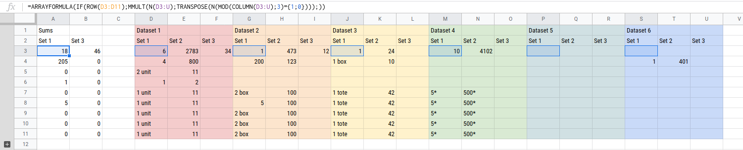
Didn't find what you were looking for?
Ask your questionAsk a Question
731 491 924 answers to any question