What actions do I need to do in the table?

Question

excel

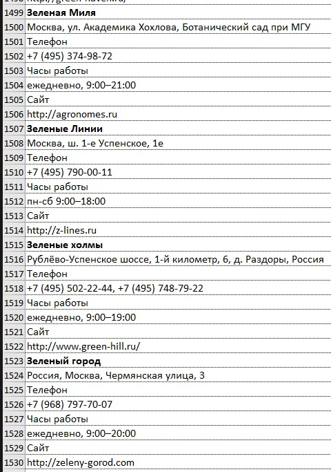
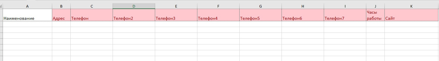
Good evening! There is a large amount of data simply written line by line (Rev. 1). You need to make the table so that only the "bold" text (which is the name of the companies) is located in the "name" column. At the same time, there are various data on the type "phone 1", "phone 2", "website". I can’t understand what formulas to choose and in general what algorithm of actions to properly set up the table (output 2)

Answer 1

If the number and type of fields are the same in the entire table, just as in your example, you can:
- insert the table from above "as is" into the table below
- for the first line with the company name, write relative links to cells with data in the appropriate columns this company, as Alexander hinted ; Daniil Babkin has in his answer a similar, but more elegant than I suggest, solution, with a universal formula for all fields
- copy these cells with formulas, paste for all other lines with the name of firms (if there are a lot of them, you can, for example, paint them in some color with a macro to filter by it with an autofilter, or make an auxiliary column and display the flag "name" with the formula firms" stupidly by the number of rows, and filter by it)
- select the entire table, copy, paste as values
​​- delete unnecessary rows - the easiest way is to use the autofilter

Answer 2

I see 2 ways - "one-time on crutches" and reusable.
For reusable sawing Powerquery query.
For disposable

1. create a column on the left (let's say column A)
   
2. filter, select all bold lines (filter by format) and put something in field A (n., number 1)
   
3. remove the filter and in the 10 fields to the right of your content, starting with field C2, insert the formula: =IF($A2=1,IF((OFFSET($A2,COUNT($B2:B2),0)="")* (COUNT($B2:B2))*(B2<>"");OFFSET($B2;COUNT($B2:B2);0);"");"")
   

The formula is given for cell C2. If your first cell is different, then just change the line number (2) to the desired one and expand the formula.
The formula is not the most elegant, but it works.
Good luck.

Answer 3

See the answer to almost the same question: How to arrange text in excel in columns?
The difference is that there the cycle was 3 lines, and you have 8 lines. Therefore, you have 10..20 seconds more manual work than there. :) But the essence is the same.

Answer 4

You need a macro that will iterate through all the lines sequentially and write (for example, to another sheet) lines with font.bold = true

Answer 5

In general, say hello to the one who led the table. I won't write a macro, but I would start with

Function ШРИФТИМЯ(ЯЧЕЙКА As Range) As String
    ШРИФТИМЯ = ЯЧЕЙКА.Font.FontStyle
End Function

It is banal that it would be possible to select the "bold" text, and from there already dance with the grouping.
But of course it's better to sit and write a macro as BasiC2k said